
Skip to content
Free Excel Tutorials
  • Home
  • Excel For Beginners
  • Excel Intermediate
  • Advanced Excel For Experts

Data Analysis

  • How to conditionally sum numeric data in an Excel table using SUMIFS
  • Conflicting Multiple Conditional Formatting Rules in Excel
  • Excel Pie Chart
  • Conditional Formatting Rules in Excel
  • Use Data Form to input, edit and delete records in Excel

References

  • How to use Excel FORMULATEXT function
  • How to calculate two-way lookup VLOOKUP in Excel Table
  • How to get relative row numbers in a range in Excel
  • How to create dynamic named range with OFFSET in Excel
  • How to get first column number in range in Excel

Data Validations

  • Excel Data validation unique values only
  • Excel Data validation allow weekday only
  • Excel Data validation allow uppercase only
  • Excel Data validation specific characters only
  • Excel Data validation number multiple 100

How to check if cell contains all of many things in Excel

by

If you want to test a cell to see if it contains all items in a list, you can do so with a formula that uses the SEARCH function, with help from the ISNUMBER, SUMPRODUCT, and COUNTA functions.

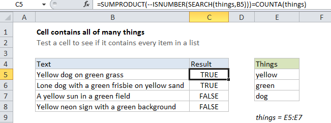
Case study: Let’s say you have a list of text strings in the range B5:B8, and you want to find out if these cells contain all of the words in another range, E5:E7.

You could build a formula that uses nested IF statements to check for each item, but that won’t scale well if you have a lot of things to look for.  Each time you add an word to look for you’ll need to add another nested IF and adjust parentheses.

Formula

=SUMPRODUCT(--ISNUMBER(SEARCH(things,A1)))=COUNTA(things)
Explanation

Solution

The solution is to to create a formula counts all matches at once. Once we have that, we simply compare that count with the count of items we’re looking for. If they match, we know a cell contains all items.

In the example shown, the formula we’re using is:

=SUMPRODUCT(--ISNUMBER(SEARCH(things,B5)))=COUNTA(things)

How this formula works

The key is this snippet:

ISNUMBER(SEARCH(things,B5)

This is based on another formula (explained in detail here) that simply checks a cell for a single substring. If the cell contains the substring, the formula returns TRUE. If not, the formula returns FALSE.

However, if we give the same formula a list of things (in this case, we are using a named range called “things”, E5:E7) it will give us back a list of TRUE / FALSE values, one for each item in . The result is an array that looks like this:

{TRUE;TRUE;TRUE}

Where each TRUE represents a found item, and each FALSE represents an item not found.

We can force the TRUE / FALSE values to 1s and 0s with a double negative (–, also called a double unary):

--ISNUMBER(SEARCH(things,B5))

which yields an array like this:

{1;1;1}

Next, we process this array with SUMPRODUCT, which will give us a total sum. If this sum is equal to the number of items in the named range “things”, we know we’ve found all things and can return TRUE. The way we do this is to compare the two numbers directly. We get a count of non-blank cells in “things” using COUNTA:

=COUNTA(things)

With a hard-coded list

There’s no requirement that you use a range for your list of things. If you’re only looking for a small number of things, you can use a list in array format, which is called an array constant. For example, if you’re just looking for the colors red, blue, and green, you can use {“red”,”blue”,”green”} like this:

=SUMPRODUCT(--ISNUMBER(SEARCH({"yellow","green","dog"},B5)))=COUNTA(things)

Post navigation

Previous Post:

DECIMAL function: Description, Usage, Syntax, Examples and Explanation

Next Post:

AVERAGE function: Description, Usage, Syntax, Examples and Explanation

Leave a Reply Cancel reply

Your email address will not be published. Required fields are marked *

Learn Basic Excel

Ribbon
Workbook
Worksheets
Format Cells
Find & Select
Sort & Filter
Templates
Print
Share
Protect
Keyboard Shortcuts

Categories

  • Charts
  • Data Analysis
  • Data Validation
  • Excel Functions
    • Cube Functions
    • Database Functions
    • Date and Time Functions
    • Engineering Functions
    • Financial Functions
    • Information Functions
    • Logical Functions
    • Lookup and Reference Functions
    • Math and Trig Functions
    • Statistical Functions
    • Text Functions
    • Web Functions
  • Excel VBA
  • Excel Video Tutorials
  • Formatting
  • Grouping
  • Others

Logical Functions

  • How to use Excel FALSE Function
  • AND function: Description, Usage, Syntax, Examples and Explanation
  • How to return blank in place of #DIV/0! error in Excel
  • FALSE function: Description, Usage, Syntax, Examples and Explanation
  • How to use Excel XOR Function

Date Time

  • Display Days in month in Excel
  • How to get same date next year or previous year in Excel
  • Get fiscal quarter from date in Excel
  • Find Last Day of the Month in Excel
  • How to determine year is a leap year in Excel

Grouping

  • Running count group by n size in Excel
  • Categorize text with keywords in Excel
  • How to randomly assign people to groups in Excel
  • Map text to numbers in Excel
  • Group numbers with VLOOKUP in Excel

General

  • How to generate random number between two numbers in Excel
  • Check if multiple cells have same value with case sensitive in Excel
  • Print Excel Sheet In Landscape Or Portrait
  • Common Errors in Excel
  • Subtotal invoices by age in Excel
© 2026 xlsoffice . All Right Reserved. | Teal Smiles | Abbreviations And Their Meaning