Count if two criteria match in Excel

This tutorial shows how to Count if two criteria match in Excel using the example below;

Formula

=COUNTIFS(range1,critera1,range2,critera2)

Explanation

If you want to count rows where two (or more) criteria match, you can use a formula based on the COUNTIFS function.

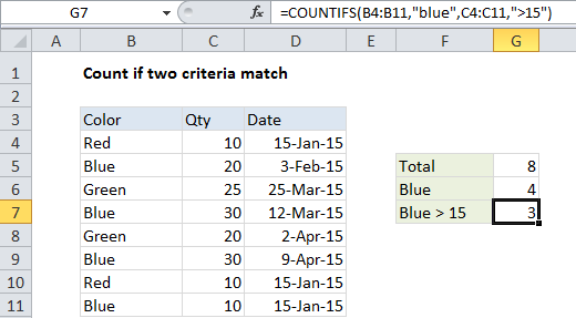
In the example shown, we want to count the number of orders with a color of “blue” and a quantity > 15. The formula we have in cell G7 is:

=COUNTIFS(B4:B11,"blue",C4:C11,">15")

How this formula works

The COUNTIFS function takes multiple criteria in pairs — each pair contains one range and the associated criteria for that range. To generate a count, all conditions must match. To add more conditions, just add another range / criteria pair.

SUMPRODUCT alternative

You can also use the SUMPRODUCT function to count rows that match multiple conditions. the equivalent formula is:

=SUMPRODUCT((B4:B11="Blue")*(C4:C11>15))

SUMPRODUCT is more powerful and flexible than COUNTIFS, and it works with all Excel versions, but it is not as fast with larger sets of data.

Pivot table alternative

If you need to summarize  number of criteria combinations in a larger data set, you should consider pivot tables. Pivot tables are a fast and flexible reporting tool that can summarize data in many different ways.