How to calculate current stock or inventory in Excel

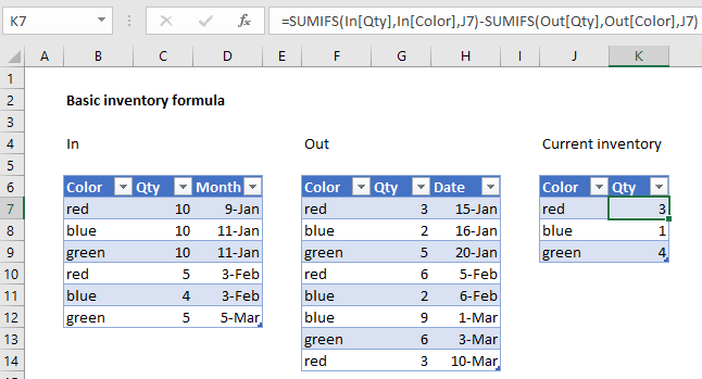
In the example shown, the formula in K7 is:

=SUMIFS(In[Qty],In[Color],J7)-SUMIFS(Out[Qty],Out[Color],J7)

Where “In” is the Excel Table on the left, “Out” is the table in the middle.

How this formula works

This formula demonstrates a very simple inventory concept where current inventory is simply the result of all incoming stock minus all outgoing stock. In the example, colors are treated as unique item identifiers – imagine a product available in one size only in just three colors: red, blue, or green.

The key to this approach is to use Excel Tables, because Table ranges automatically expand to handle changes in data. This means we can get a total of all incoming red items with:

=SUMIFS(In[Qty],In[Color],J7)

And a total of all outgoing red items with:

=SUMIFS(Out[Qty],Out[Color],J7)

In both cases, the SUMIFS function generates a total for all red items in each table.

Then, as long as both tables are up to date and complete, we can get the current inventory of red items with the following formula:

=SUMIFS(In[Qty],In[Color],J7)-SUMIFS(Out[Qty],Out[Color],J7)

As the formula is copied down, we get current inventory for each color.