Skip to content
Free Excel Tutorials
  • Home
  • Excel For Beginners
  • Excel Intermediate
  • Advanced Excel For Experts

Data Analysis

  • Calculate Conditional Percentile ‘IF’ in table in Excel
  • Example of COUNTIFS with variable table column in Excel
  • Conflicting Multiple Conditional Formatting Rules in Excel
  • How to conditionally sum numeric data in an Excel table using SUMIFS
  • How to create Gauge Chart in Excel

References

  • How to use Excel ROW Function
  • Count unique text values with criteria
  • MATCH function: Description, Usage, Syntax, Examples and Explanation
  • How to use Excel LOOKUP Function
  • Get nth match with INDEX / MATCH in Excel

Data Validations

  • Excel Data validation allow uppercase only
  • Excel Data validation only dates between
  • Data validation must not exist in list
  • Excel Data validation must begin with
  • Excel Data validation allow weekday only

Match next highest value in Excel

by

This tutorial shows how to Match next highest value in Excel using the example below;

Formula

=INDEX(data,MATCH(lookup,values)+1)

Explanation

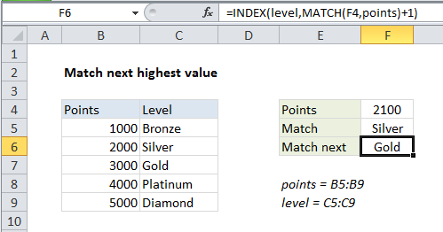
To match the “next highest” value in a lookup table, you can use a formula based on INDEX and MATCH. In the example shown, the formula in F6 is:

=INDEX(level,MATCH(F4,points)+1)

where “level” is the named range C5:C9, and “points” is the named range B5:B9.

How this formula works

This formula is a standard version of INDEX + MATCH with a small twist.

Working from the inside out, MATCH is used find the correct row number for the value in F4, 2100. Without the third argument, match_type, defined, MATCH defaults to approximate match and returns 2.

The small twist is that we add 1 to this result to override the matched result and return 3 as the row number for INDEX.

With level (C5:C9) supplied as the array, and 3 as the row number, INDEX returns “Gold”:

=INDEX(level,3) // returns Gold

Another option

The above approach works fine for simple lookups. If you want to use MATCH to find the “next largest” match in more traditional way, you can sort the lookup array in descending order, and use MATCH as described on this page.

Post navigation

Previous Post:

How to use Excel CHOOSE Function

Next Post:

Customize Ribbon In Excel

Leave a Reply Cancel reply

Your email address will not be published. Required fields are marked *

Learn Basic Excel

Ribbon
Workbook
Worksheets
Format Cells
Find & Select
Sort & Filter
Templates
Print
Share
Protect
Keyboard Shortcuts

Categories

  • Charts
  • Data Analysis
  • Data Validation
  • Excel Functions
    • Cube Functions
    • Database Functions
    • Date and Time Functions
    • Engineering Functions
    • Financial Functions
    • Information Functions
    • Logical Functions
    • Lookup and Reference Functions
    • Math and Trig Functions
    • Statistical Functions
    • Text Functions
    • Web Functions
  • Excel VBA
  • Excel Video Tutorials
  • Formatting
  • Grouping
  • Others

Logical Functions

  • How to use Excel OR Function
  • IFERROR function: Description, Usage, Syntax, Examples and Explanation
  • Return blank if in Excel
  • Extract multiple matches into separate rows in Excel
  • NOT function: Description, Usage, Syntax, Examples and Explanation

Date Time

  • How to calculate working days left in month in Excel
  • Get first day of previous month in Excel
  • Calculate series of dates by workdays in Excel
  • TODAY function: Description, Usage, Syntax, Examples and Explanation
  • Convert decimal seconds to Excel time

Grouping

  • Map text to numbers in Excel
  • Group numbers with VLOOKUP in Excel
  • Group arbitrary text values in Excel
  • Group times into unequal buckets in Excel
  • Group times into 3 hour buckets in Excel

General

  • How to calculate percent sold in Excel
  • How to test a range for numbers in Excel
  • Count cells that contain errors in Excel
  • How to count total columns in range in Excel
  • Count cells that do not contain errors in Excel
© 2026 xlsoffice . All Right Reserved. | Teal Smiles | Abbreviations And Their Meaning