
Skip to content
Free Excel Tutorials
  • Home
  • Excel For Beginners
  • Excel Intermediate
  • Advanced Excel For Experts

Data Analysis

  • Subtotal function in Excel
  • How to count table columns in Excel
  • Chart Axes in Excel
  • How to combine 2 or more chart types in a single chart in Excel
  • How to create a Histogram in Excel

References

  • How to use Excel MATCH Function
  • How to reference named range different sheet in Excel
  • Get nth match with INDEX / MATCH in Excel
  • Offset in Excel
  • How to get last row in text data in Excel

Data Validations

  • Excel Data validation allow uppercase only
  • Excel Data validation date in specific year
  • Excel Data validation don’t exceed total
  • Excel Data validation no punctuation
  • Excel Data validation specific characters only

Two-way lookup with VLOOKUP in Excel

by

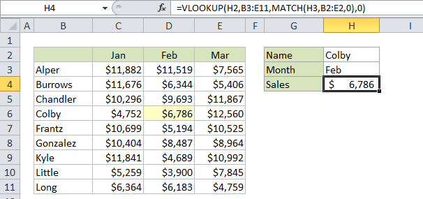
This tutorial shows how to calculate Two-way lookup with VLOOKUP in Excel  using the example below;

Formula

=VLOOKUP(lookup_value,table,MATCH(col_name,col_headers,0),0)
Explanation

Note:

Inside the VLOOKUP function, the column index argument is normally hard-coded as a static number. However, you can also create a dynamic column index by using the MATCH function to locate the right column. This technique allows you to create a dynamic two-way lookup, matching on both rows and columns. It can also make a VLOOKUP formula more resilient: VLOOKUP can break when columns are inserted or removed from a table, but a formula with VLOOKUP + MATCH can continue to work correctly even changes are made to columns.

Example

In the example, we are using this formula to dynamically lookup both rows and columns with VLOOKUP:

=VLOOKUP(H2,B3:E11,MATCH(H3,B2:E2,0),0)

H2 supplies the lookup value for the row, and H3 supplies the lookup value for the column.

How this formula works

This is a standard VLOOKUP exact match formula with one exception: the column index is supplied by the MATCH function.

Note that the lookup array given to MATCH (B2:E2) representing column headers deliberately includes the empty cell B2. This is done so that the number returned by MATCH is in sync with the table used by VLOOKUP. In other words, you need to give MATCH a range that spans the same number of columns VLOOKUP is using in the table. In the example (for Feb) MATCH returns 3, so after MATCH runs, the VLOOKUP formula looks like this:

=VLOOKUP(H2,B3:E11,3,0)

Which returns sales for Colby (row 4) in Feb (column 3), which is $6,786.

Post navigation

Previous Post:

COSH function: Description, Usage, Syntax, Examples and Explanation

Next Post:

Excel Data validation require unique number

Leave a Reply Cancel reply

Your email address will not be published. Required fields are marked *

Learn Basic Excel

Ribbon
Workbook
Worksheets
Format Cells
Find & Select
Sort & Filter
Templates
Print
Share
Protect
Keyboard Shortcuts

Categories

  • Charts
  • Data Analysis
  • Data Validation
  • Excel Functions
    • Cube Functions
    • Database Functions
    • Date and Time Functions
    • Engineering Functions
    • Financial Functions
    • Information Functions
    • Logical Functions
    • Lookup and Reference Functions
    • Math and Trig Functions
    • Statistical Functions
    • Text Functions
    • Web Functions
  • Excel VBA
  • Excel Video Tutorials
  • Formatting
  • Grouping
  • Others

Logical Functions

  • How to use Excel OR Function
  • Return blank if in Excel
  • IFNA function: Description, Usage, Syntax, Examples and Explanation
  • SWITCH function: Description, Usage, Syntax, Examples and Explanation
  • Invoice status with nested if in Excel

Date Time

  • How to calculate most recent day of week in Excel
  • Get work hours between dates in Excel
  • Convert date to text in Excel
  • How to get Holiday Date from Year in Excel
  • Display the current date in Excel

Grouping

  • If cell contains one of many things in Excel
  • Group numbers with VLOOKUP in Excel
  • Categorize text with keywords in Excel
  • Map inputs to arbitrary values in Excel
  • Group times into 3 hour buckets in Excel

General

  • List sheet names with formula in Excel
  • With vs Without Array Formula in Excel
  • How to Create Calendar in Excel
  • Excel Ribbon Quick Overview For Beginners
  • Convert column letter to number in Excel
© 2026 xlsoffice . All Right Reserved. | Teal Smiles | Abbreviations And Their Meaning