Join tables with INDEX and MATCH in Excel

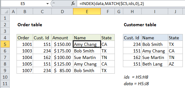
To join or merge tables that have a common id, you can use the INDEX and MATCH functions. In the example shown, the formula in E5 is:

=INDEX(data,MATCH($C5,ids,0),2)

where “data” is the named range H5:J8 and “ids” is the named range H5:H8.

How this formula works

This formula pulls the customer name and state from the customer table into the order table. The MATCH function is used to locate the right customer and the INDEX function is used to retrieve the data.

Retrieving customer name

Working from the inside out, the MATCH function is used to get a row number like this:

MATCH($C5,ids,0)

• The lookup value comes the customer id in C5, which is a mixed reference, with the column locked, so the formula can be easily copied.
• The lookup array is the named range ids (H5:H8), the first column in the customer table.
• The match type is set to zero to force an exact match.

The MATCH function returns 2 in this case, which goes into INDEX as the row number:

=INDEX(data,2,2)

With the column number hard-coded as 2 (customer names are in column 2) and the array set to the named range “data” (H5:J8) INDEX returns: Amy Chang.

Retrieving customer state

The formula to retrieve customer state is almost identical. The only difference is the column number is hard-coded as 3, since state info appears in the 3rd column:

=INDEX(data,MATCH($C5,ids,0),2) // get name
=INDEX(data,MATCH($C5,ids,0),3) // get state

Dynamic two-way match

By adding another MATCH function to the formula, you can set up a dynamic two-way match. For example, with the named range “headers” for  H4:J4, you can use a formula like this:

=INDEX(data,MATCH($C5,ids,0),MATCH(E$4,headers,0))

Here, a second MATCH function has been added to get the correct column number. MATCH uses the current column header in the first table to locate the correct column number in the second table, and automatically returns this number to INDEX.