Count cells not equal to many things in Excel

This tutorial shows how to Count cells not equal to many things in Excel using the example below;

Formula

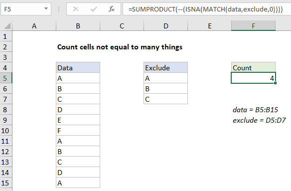
=SUMPRODUCT(--(ISNA(MATCH(data,exclude,0))))

Explanation

To count cells not equal to any of many things, you can use a formula based on the MATCH, ISNA, and SUMPRODUCT functions. In the example shown, the formula in cell F5 is:

=SUMPRODUCT(--(ISNA(MATCH(data,exclude,0))))

where “data” is the named range B5:B16 and “exclude” is the named range D5:D7.

How this formula works

First, a little context. Normally, if you have just a couple things you don’t want to count, you can COUNTIFS like this:

=COUNTIFS(range,"<>apple",range,"<>orange")

But this doesn’t scale very well if you have a list of many things, because you’ll have to add an additional range/criteria pair to for each thing you don’t want to count. It would be a lot easier to build a list and pass in a reference to this list as part of the criteria. That’s exactly what the formula on this page does.

At the core, this formula uses the MATCH function to find cells not equal to “a”,  “b”, or “c” with this expression:

MATCH(data,exclude,0)

Note the lookup value and lookup array are “reversed” from normal configuration — we provide all values from the named range “data” as lookup values, and give all values we want to exclude in the named range “exclude”. Because we give MATCH more than one lookup value, we get more than one result in an array like this:

{1;2;3;#N/A;#N/A;#N/A;1;2;3;#N/A;1}

Essentially, MATCH gives us the position of matching values as a number, and returns #N/A for all other values.

The #N/A results are the ones we’re interested in, since they represent values not equal to “a”,  “b”, or “c”. Accordingly, we use ISNA to force these values to TRUE, and the numbers to FALSE:

ISNA(MATCH(data,exclude,0)

Then we use a double negative to coerce TRUE to 1 and FALSE to zero. The resulting array, inside SUMPRODUCT looks like this:

=SUMPRODUCT({0;0;0;1;1;1;0;0;0;1;0})

With only one array to process, SUMPRODUCT sums and returns a final result, 4.

Note: Using SUMPRODUCT instead of SUM avoids the need to use control + shift + enter.

Count minus match

Another way to count cells not equal to any of several things is to count all values, and subtract matches. You can do this with a formula like this:

=COUNTA(range)-SUMPRODUCT(COUNTIF(range,exclude))

Here, COUNTA returns a count of all non-empty cells. The COUNTIF function, given the named range “exclude” will return three counts, one for each item in the list. SUMPRODUCT adds up the total, and this number is subtracted from the count of all non-empty cells. The final result is the number of cells that do not equal values in “exclude”.

Literal contains type logic

The formula on this page counts with “equals to” logic. If you need to count cells that do not contain many strings, where contains means a string may appear anywhere in a cell, you’ll need a more complex formula.