Sum range with INDEX in Excel

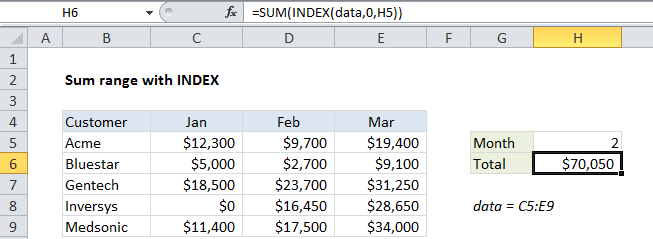
This tutorial shows how to calculate Sum range with INDEX in Excel using the example below;

 Formula

=SUM(INDEX(data,0,column))

Explanation

To sum all values in a column or row, you can use the INDEX function to retrieve the values, and the SUM function to return the sum.  This technique is useful in situations where the row or column being summed is dynamic, and changes based on user input.  In the example shown, the formula in H6 is:

=SUM(INDEX(data,0,H5))

where “data” is the named range C5:E9.

How this formula works

The INDEX function looks up values by position. For example, this formula retrieves the value for Acme sales in Jan:

=INDEX(data,1,1)

The INDEX function has a special and non-obvious behavior: when the row number argument is supplied as zero or null, INDEX retrieves all values in the column referenced by the column number argument. Likewise, when the column number is supplied as zero or nothing, INDEX retrieves all values in the row referenced by the row number argument:

=INDEX(data,0,1) // all of column 1
=INDEX(data,1,0) // all of row 1

In the example for formula, we supply the named range “data” for array, and we pick up the column number from H2. For row number, we deliberately supply zero. This causes INDEX to retrieve all values in column 2 of “data’. The formula is solved like this:

=SUM(INDEX(data,0,2))
=SUM({9700;2700;23700;16450;17500})
=70050

Other calculations

You can use the same approach for other calculations by replacing SUM with AVERAGE, MAX, MIN, etc. For example, to get an average of values in the third month, you can use:

=AVERAGE(INDEX(data,0,3))