Exact match lookup with SUMPRODUCT in Excel

Case sensitive lookups in Excel

By default, standard lookups in Excel are not case-sensitive. Both VLOOKUP and INDEX/MATCH will simply return the first match, ignoring case.

A direct way to workaround this limitation, is to use an array formula based on INDEX/MATCH with EXACT. However, if you’re looking up numeric values only, SUMPRODUCT + EXACT also gives an interesting and flexible way to do a case-sensitive lookup.

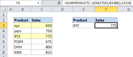
In the example, we are using the following formula

=SUMPRODUCT(--(EXACT(E3,B3:B8)),C3:C8)

Although this formula is an array formula, it does not need to be entered with Control + Shift + Enter, since SUMPRODUCT handles arrays natively.

How the formula works

SUMPRODUCT is designed to work with arrays, which it multiplies, then sums.

In this case, we are two arrays with SUMPRODUCT: B3:B8 and C3:C8. The trick is to run a test on the values in column B, then convert the resulting TRUE/FALSE values to 1’s and 0’s. We run the test with EXACT like so:

EXACT(E3,B3:B8)

Which produces this array:

{FALSE;FALSE;TRUE;FALSE;FALSE;FALSE}

Note that the true value in position 3 is our match. Then we use the double negative (i.e. –, which is technically a “double unary”) to coerce these TRUE / FALSE values into 1 and 0. The result is this array:

{0;0;1;0;0;0}

At this point in the calculation, the SUMPRODUCT formula looks like this:

=SUMPRODUCT({0;0;1;0;0;0},{875;750;775;675;800;825})

SUMPRODUCT then simply multiples the items in each array together to produce a final array:

{0;0;775;0;0;0}

Which SUMPRODUCT then sums, and returns 775.

So, the gist of this formula is that the FALSE values are used to cancel out all other values. The only values that survive are those that were TRUE.

Note that because we are using SUMPRODUCT, this formula comes with a unique twist: if there are multiple matches, SUMPRODUCT will return the sum of those matches. This may or may not be what you want, so take care if you do expect multiple matches!

Remember, this formula only works for numeric values, because SUMPRODUCT does’t handle text. If you want to retrieve text, use  INDEX/MATCH + EXACT.