Format Cells and Numbers in Excel
Format Cells simply refers to style; font, font colour, font size, borders and more while Format Numbers refer to data pattern, ie percentage, currency and more.
Format Numbers
We can apply a number format (0.8, $0.80, 80%, etc) or other formatting (alignment, font, border, etc).
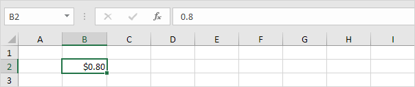
1. Enter the value 0.8 into cell B2.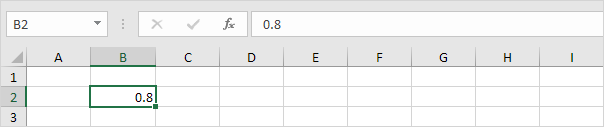
By default, Excel uses the General format (no specific number format) for numbers. To apply a number format, use the ‘Format Cells’ dialog box.
2. Select cell B2.
3. Right click, and then click Format Cells (or press CTRL + 1).
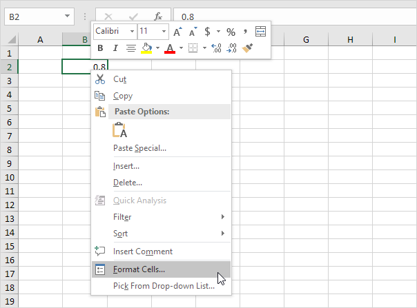
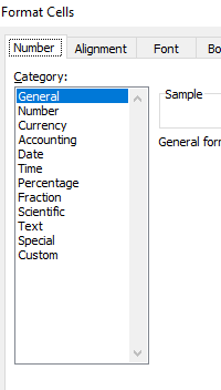
The ‘Format Cells’ dialog box appears.
4. For example, select Currency.
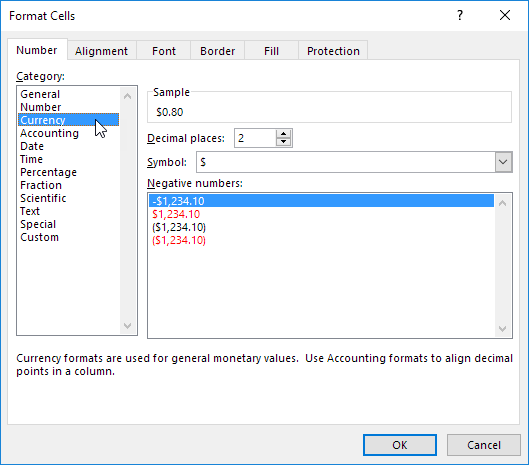
Note: Excel gives you a life preview of how the number will be formatted (under Sample).
5. Click OK.
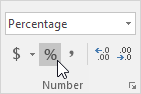
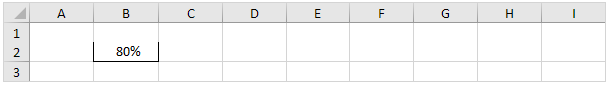
6. On the Home tab, in the Number group, click the percentage symbol to apply a Percentage format.
Format Cells
Cell B2 still contains the number 0.8. We only changed the appearance of this number. The most frequently used formatting commands are available on the Home tab.
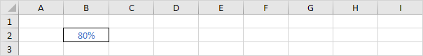
7. On the Home tab, in the Alignment group, center the number.

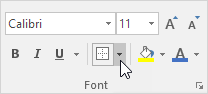
8. On the Home tab, in the Font group, add outside borders and change the font color to blue.
Result:
See more examples on how to use excel number format.
In Microsoft Excel, there are several formats available when dealing with numeric data.
It always makes a difference to have your data formatted for viewing.
But this isn’t the primary reason for number formatting. Not all number formats the same in form or function.
If you are working with percentages, integers or currency format will not work well.
Formatting your data using number formats is quite simple.
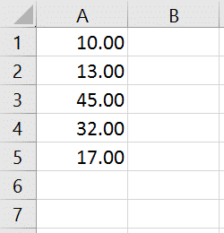
The first thing to do is highlight the data. Then go to the Number group on the Home tab.
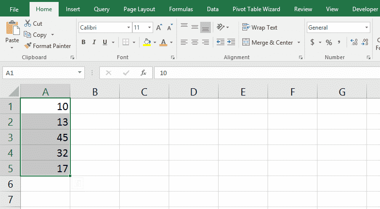
By default, number data that you enter is in General format until you change it.
The next thing to do is click on the small down arrow next to “General.”
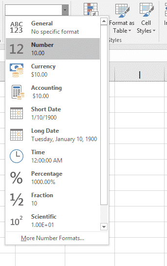
If you click on Number, Excel changes your values to that format. You should now see your data with two decimal places added.
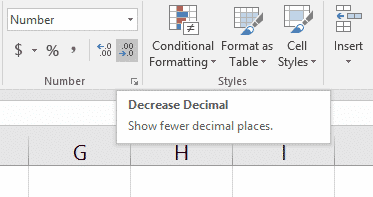
To remove those decimal places, select the data and go to the Number section of the Home tab again.
You can then click Decrease Decimal a couple of times.
You could also change the number format of your data to currency. Select Currency from the drop-down list.
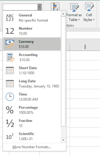
This will now change your data accordingly.

You can get even more detailed with your number formatting. Click the small angled arrow in the lower right hand corner of the Number group.
This will expand the Number Format group.
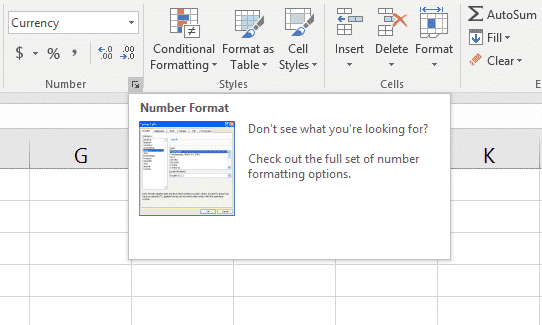
This will open the Format Cells dialog box. You will find many options available here.
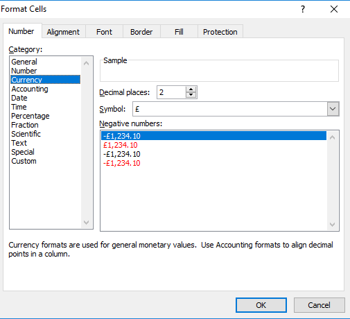
This is where you can do things like set decimal places and how you want negative numbers to appear.
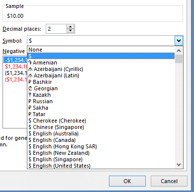
You can even change the symbol of the currency based on your needs.
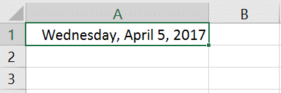
Let’s look at an example about date data. Say you have a date in the following format.
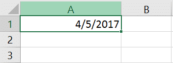
Select the cell containing the date.
Open the Format Cells dialog box and select Date from the Categories list.
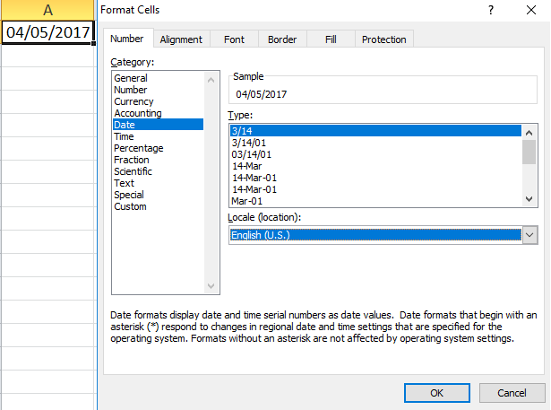
Notice the many format variations in the Type list. Another thing to note is the sample shown above Type.
It gives you a quick glance at your actual data in the selected format type.
This will change as you cycle through the various types giving you a quick preview. Let’s select the long date format or the second type selection from the top.
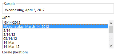
We can see a preview in the Sample window. We must click OK to reformat our data.