Lookup entire column in Excel

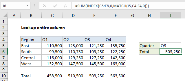
To lookup and retrieve an entire column, you can use a formula based on the INDEX and MATCH functions. In the example shown, the formula used to lookup all Q3 results is:

=INDEX(C5:F8,0,MATCH(I5,C4:F4,0))

Note: this formula is embedded in the SUM function only to demonstrate that all values are correctly retrieved.

How this formula works

The gist: use MATCH to identify the column index, then INDEX to retrieve the entire column by setting the row number to zero.

Working from the inside out, MATCH is used to get the column index like this:

MATCH(I5,C4:F4,0)

The lookup value “Q3” comes from H5, the array is the headers in C4:F4, and zero is used to force an exact match. The MATCH function returns 3 as a result, which is fed into the INDEX function as the column number.

Inside INDEX, the array is provided as the range C5:F8, and the column number is 3, as provided by MATCH. Row number is set to zero:

=INDEX(C5:F8,0,3)

This causes INDEX to return all 4 values in of the array as the final result, in an array like this:

{121250;109250;127250;145500}

In the example shown, the entire formula is wrapped in the SUM function, which can handle arrays natively. The SUM function returns a final result of 503,250.

Processing with other functions

Once you retrieve an entire column of data, you can feed that column into functions like SUM, MAX, MIN, AVERAGE, LARGE, etc. for additional processing. For example, you could get the maximum value in a quarter like this:

=MAX(INDEX(C5:F8,0,MATCH(I5,C4:F4,0)))