Count numbers third digit equals 3 in Excel

This tutorial shows how to Count numbers third digit equals 3 in Excel using the example below;

Formula

=SUMPRODUCT(--(MID(range,3,1)="3"))

Explanation

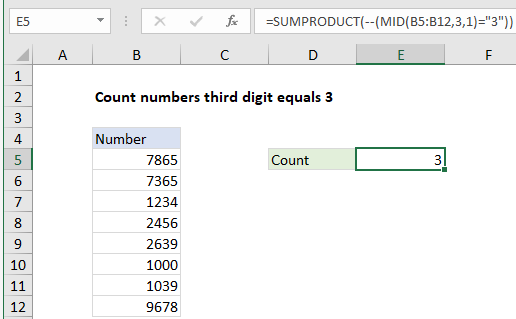
To count numbers where the third digit equals 3, you can use a formula based on the SUMPRODUCT and MID functions. In the example shown, the formula in E5 is:

=SUMPRODUCT(--(MID(B5:B12,3,1)="3"))

How this formula works

To get the third character from a string in A1, you can use the MID function like this:

=MID(A1,3,1)

The first argument is a cell reference, the second argument specifies the start number, and the third argument indicates number of characters.

If you give the MID function a range of cells for the first argument, you’ll get back an array of results. In the example shown, this expression:

MID(B5:B12,3,1)

returns an array like this:

{"6";"6";"3";"5";"3";"0";"3";"7"}

This array contains the third digit from each cell in the range B5:B12. Notice the MID function has automatically converted numeric values in the range to text strings and returned the third character as a text value.

When we compare this array using =”3″, we get an array like this:

{FALSE;FALSE;TRUE;FALSE;TRUE;FALSE;TRUE;FALSE}

We use the double negative to coerce the TRUE and FALSE values to 1 and zero respectively, which returns:

{0;0;1;0;1;0;1;0}

Finally, with only one array to work with, the SUMPRODUCT function sums the items in the array and returns the total, 3.