Highlight rows with blank cells in Excel

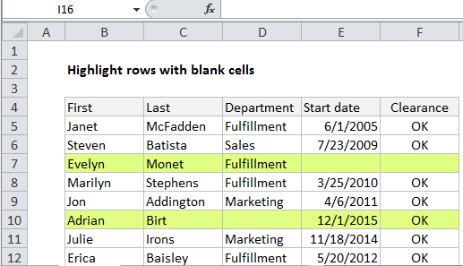
This tutorial shows how to Highlight rows with blank cells in Excel using the example below;

Formula

=COUNTBLANK($B5:$F5)

Explanation

To highlight rows that contain one or more blank cells. you can conditional formatting with a simple formula based on the COUNTBLANK function.

In the example shown, the range B5:F15 is formatted with a conditional formatting rule based on this formula:

=COUNTBLANK($B5:$F5)

Note: it’s important that CF formulas be entered relative to the “first cell” in the selection, B5 in this case.

Once you save the rule, you’ll see the rows that contain one or more blank cells highlighted.

How this formula works

Conditional formatting is applied to all cells in the active selection at the time a rule is created.

In this case, the column references are locked to prevent columns from changing as the formula is evaluated, but the row references are relative so that row numbers are free to change. The result is a formula that applies exactly the same logic to every cell in the same row.

If COUNTBLANK finds any blank cells in a given row, it returns a positive number, which Excel evaluates to TRUE,  triggering the rule.

If COUNTBLANK finds no blank cells, it returns zero, which is evaluated as FALSE, and the formatting is not triggered.