Highlight missing values in Excel

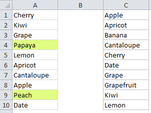
To compare lists and highlight values that exist in one but not the other,  you can apply conditional formatting with a formula based on the COUNTIF function. For example, to highlight values A1:A10 that don’t exist C1:C10, select A1:A10 and create a conditional formatting rule based on this formula:

=COUNTIF($C$1:$C$10,A1)=0

Note: with conditional formatting, it’s important to enter the formula relative to the “active cell” in the selection, which is assumed to be A1 in this case.

How this formula works

This formula is evaluated for each of the 10 cells in A1:D10. A1 will change to the address of the cell being evaluated, while C1:C10 is entered as an absolute address, so it won’t change at all.

The key to this formula is the =0 at the end, which “flips” the logic of the formula. For each value in A1:A10,  COUNTIF returns the number of times the value appears in C1:C10. As long as the value appears at least once in C1:C10, COUNTIF will return a non-zero number and the formula will return FALSE.

But when a value is not found in C1:C10, the COUNTIF returns zero and, since 0 = 0, the formula will return TRUE and the conditional formatting will be applied.

Named ranges for simple syntax

If you name the list you are searching (C1:C10 in this case) with a named range, the formula is simpler to read and understand:

=COUNTIF(list,A1)=0

This works because named ranges are automatically absolute.

Case-sensitive version

If you need a case sensitive count, you can use a formula like this:

=SUMPRODUCT((--EXACT(A1,list)))=0

The EXACT function performs a case-sensitive evaluation and SUMPRODUCT tallies the result. As with the COUNTIF, this formula will return when the result is zero. Because the test is case-sensitive, “apple” will show as missing even if “Apple” or “APPLE” appears in the second list. See this page for a more detailed explanation.