Skip to content
Free Excel Tutorials
  • Home
  • Excel For Beginners
  • Excel Intermediate
  • Advanced Excel For Experts

Data Analysis

  • Excel Pie Chart
  • Excel Bar Chart
  • Conditional Formatting Data bars Examples in Excel
  • How to add Trendline to a chart in Excel
  • Conditional Formatting Rules in Excel

References

  • How to get first row number in range in Excel
  • How to get relative column numbers in a range in Excel
  • Complete List of Excel Lookup and Reference Functions, References and Examples
  • Find closest match in Excel
  • VLOOKUP function: Description, Usage, Syntax, Examples and Explanation

Data Validations

  • Excel Data validation must not contain
  • Excel Data validation don’t exceed total
  • Data validation must not exist in list
  • How To Create Drop-down List in Excel
  • Excel Data validation only dates between

How to get top level domain (TLD) in Excel

by

To extract the top level domain (called “TLD”)  from a list of domain names or email addresses, you can use a rather complex formula that uses several functions. In the formula below, domain represents a domain or email address in normal “dot” syntax.

Formula

=RIGHT(domain,LEN(domain)-FIND("*",SUBSTITUTE(domain,".","*",
LEN(domain)-LEN(SUBSTITUTE(domain,".","")))))

Explanation

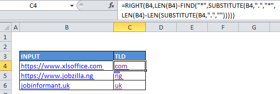
In the example, the active cell contains this formula:

=RIGHT(B4,LEN(B4)-FIND("*",SUBSTITUTE(B4,".","*",LEN(B4)-LEN(SUBSTITUTE(B4,".","")))))

How the formula works:

At the core, this formula uses the RIGHT function to extract characters starting from the right.

The other functions in this formula just do one thing: they figure out how many characters need to be extracted.

At a high level, the formula replaces the last dot “.” in the domain with an asterisk “*” and then uses FIND to locate the position of the asterisk. Once the position is known, the RIGHT function can extract the TLD.

You may wonder how the formula knows to replace only the last dot?

This is the clever part of the formula.

The key is this part:

SUBSTITUTE(B4,".","*",LEN(B4)-LEN(SUBSTITUTE(B4,".","")))

which does the actual replacement of the last dot with “*”.

The trick is that SUBSTITUTE has a forth (optional) argument that specifies which “instance” of the find text should be replaced. If nothing is supplied for this argument, all instances are replaced. However, if, say the number 2 is supplied, only the second instance is replaced.

So, the formula needs to figure out which instance to replace, which is done here:

LEN(B4)-LEN(SUBSTITUTE(B4,".",""))

The length of the domain without any dots is subtracted from the full length of the domain. The result is the number of dots in the domain.

In the example name in B4, there are two dots in the domain, so the number 2 is used as in the instance number:

SUBSTITUTE(B4," ","*",2)

This replaces only second dot with “*”. The name then looks like this:

“www.domain*com”

The FIND function then takes over to figure out exactly where the asterisk is in the text:

FIND("*", "www.domain*com")

The result is 11 (the * is in the 11th position) which is subtracted from the total length of the domain:

LEN(B4)-11

Since the name is 15 characters, we have:

14-11 = 3

Finally, the number 3 is used by RIGHT like so:

=RIGHT(B4,3)

Which results in “com”

So there you have it. That’s how this formula extracts only the top level domain from a full domain name or email address.

Post navigation

Previous Post:

DECIMAL function: Description, Usage, Syntax, Examples and Explanation

Next Post:

AVERAGE function: Description, Usage, Syntax, Examples and Explanation

Leave a Reply Cancel reply

Your email address will not be published. Required fields are marked *

Learn Basic Excel

Ribbon
Workbook
Worksheets
Format Cells
Find & Select
Sort & Filter
Templates
Print
Share
Protect
Keyboard Shortcuts

Categories

  • Charts
  • Data Analysis
  • Data Validation
  • Excel Functions
    • Cube Functions
    • Database Functions
    • Date and Time Functions
    • Engineering Functions
    • Financial Functions
    • Information Functions
    • Logical Functions
    • Lookup and Reference Functions
    • Math and Trig Functions
    • Statistical Functions
    • Text Functions
    • Web Functions
  • Excel VBA
  • Excel Video Tutorials
  • Formatting
  • Grouping
  • Others

Logical Functions

  • Invoice status with nested if in Excel
  • IF function: Description, Usage, Syntax, Examples and Explanation
  • XOR function: Description, Usage, Syntax, Examples and Explanation
  • Nested IF function example in Excel
  • How to use IFS function in Excel

Date Time

  • Series of dates by day
  • Get first day of previous month in Excel
  • Get first day of month in Excel
  • YEARFRAC function: Description, Usage, Syntax, Examples and Explanation
  • Get age from birthday in Excel

Grouping

  • Group numbers at uneven intervals in Excel
  • If cell contains one of many things in Excel
  • Map text to numbers in Excel
  • Running count group by n size in Excel
  • Group arbitrary text values in Excel

General

  • With vs Without Array Formula in Excel
  • Transpose: Switch ‘Rows to Columns’ or ‘Columns to Rows’ in Excel
  • How to get amount with percentage in Excel
  • Basic error trapping example in Excel
  • Common Errors in Excel
© 2025 xlsoffice . All Right Reserved. | Teal Smiles | Abbreviations And Their Meaning