Skip to content
Free Excel Tutorials
  • Home
  • Excel For Beginners
  • Excel Intermediate
  • Advanced Excel For Experts

Data Analysis

  • How to create Checklist in Excel
  • Excel Frequency Function Example
  • Create Scatter Chart in Excel
  • How to Create Thermometer Chart in Excel
  • How To Remove Duplicates In Excel Column Or Row?

References

  • Last row number in range
  • INDEX function: Description, Usage, Syntax, Examples and Explanation
  • Count rows with at least n matching values
  • Find closest match in Excel
  • How to use Excel ROW Function

Data Validations

  • Excel Data validation date in specific year
  • Excel Data validation number multiple 100
  • Excel Data validation must not contain
  • Excel Data validation require unique number
  • Excel Data validation allow weekday only

How to check cell equals one of many things in Excel

by

If you want to test a cell to see if it equals one of several things, you can do so with a formula that uses the SUMPRODUCT function.

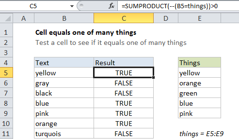
Case study:  Let’s say you have a list of text strings in the range B5:B11, and you want to test each cell against another list of things in range E5:E9. In other words, for each cell in B5:B11, you want to know: does this cell equal any of the things in E5:E9?

You could start build a big formula based on nested IF statements, but an array formula based on SUMPRODUCT is a simpler, cleaner approach.

Formula

=SUMPRODUCT(--(A1=things))>0

Explanation

The solution is to to create a formula that will test for multiple values and return a list of TRUE / FALSE values. Once we have that, we can process that list (an array, actually) with SUMPRODUCT.

The formula we’re using looks like this:

=SUMPRODUCT(--(B5=things))>0

How this formula works

The key is this snippet:

--(B5=things)

which simply compares the value in B5 to every value in the named range “things”. Because we are comparing B5 to an array (i.e. the named range “things”, E5:E11) the result will be an array of TRUE / FALSE values like this:

{TRUE;FALSE;FALSE;FALSE;FALSE}

If we have even one TRUE in the array, we know that B5 equals at least one thing in the list, so, to force the TRUE / FALSE values to 1s and 0s, we use a double negative (–, also called a double unary). After this coercion, we have this:

{1;0;0;0;0}

Now we process the result with SUMPRODUCT, which will add up the elements in the array. If we get any non-zero result, we have at least one match, so we use >1 to force a final result of either TRUE or FALSE.

With a hard-coded list

There’s no requirement that you use a range for your list of things. If you’re only looking for a small number of things, you can use a list in array format, which is called an array constant. For example, if you’re just looking for the colors red, blue, and green, you can use {“red”,”blue”,”green”} like this:

--(B5={"red","blue","green"})

Dealing with extra spaces

If the cells you are testing contain any extra space, they won’t match properly. To strip all extra space, you can modify the formula to use the TRIM function like so:

=SUMPRODUCT(--(TRIM(A1)=things))>0

Post navigation

Previous Post:

DECIMAL function: Description, Usage, Syntax, Examples and Explanation

Next Post:

AVERAGE function: Description, Usage, Syntax, Examples and Explanation

Leave a Reply Cancel reply

Your email address will not be published. Required fields are marked *

Learn Basic Excel

Ribbon
Workbook
Worksheets
Format Cells
Find & Select
Sort & Filter
Templates
Print
Share
Protect
Keyboard Shortcuts

Categories

  • Charts
  • Data Analysis
  • Data Validation
  • Excel Functions
    • Cube Functions
    • Database Functions
    • Date and Time Functions
    • Engineering Functions
    • Financial Functions
    • Information Functions
    • Logical Functions
    • Lookup and Reference Functions
    • Math and Trig Functions
    • Statistical Functions
    • Text Functions
    • Web Functions
  • Excel VBA
  • Excel Video Tutorials
  • Formatting
  • Grouping
  • Others

Logical Functions

  • IFERROR function: Description, Usage, Syntax, Examples and Explanation
  • Extract multiple matches into separate rows in Excel
  • How to use Excel NOT Function
  • Nested IF function example in Excel
  • IF, AND, OR and NOT Functions Examples in Excel

Date Time

  • How to get same date next year or previous year in Excel
  • Count times in a specific range in Excel
  • Calculate years between dates in Excel
  • NETWORKDAYS.INTL function: Description, Usage, Syntax, Examples and Explanation
  • Basic timesheet formula with breaks in Excel

Grouping

  • Group times into 3 hour buckets in Excel
  • How to randomly assign people to groups in Excel
  • How to randomly assign data to groups in Excel
  • Group numbers with VLOOKUP in Excel
  • Group times into unequal buckets in Excel

General

  • How to calculate percentage discount in Excel
  • How to create dynamic named range with INDEX in Excel
  • How to fill cell ranges with random number from fixed set of options in Excel
  • How to fill cell ranges with random text values in Excel
  • Index and match on multiple columns in Excel
© 2025 xlsoffice . All Right Reserved. | Teal Smiles | Abbreviations And Their Meaning