Highlight cells that contain one of many in Excel

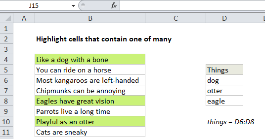
This tutorial shows how to Highlight cells that contain one of many in Excel using the example below;

Formula

=SUMPRODUCT(--ISNUMBER(SEARCH(things,A1)))>0

Explanation

To highlight cells that contain one of many text strings, you can use a formula based on the functions ISNUMBER and SEARCH, together with the SUMPRODUCT function. In the example shown, the conditional formatting applied to B4:B11 is based on this formula:

=SUMPRODUCT(--ISNUMBER(SEARCH(things,B4)))>0

How this formula works

Working from the inside out, this part of the formula searches each cell in B4:B11 for all values in the named range “things”:

--ISNUMBER(SEARCH(things,B4)

The SEARCH function returns the position of the value if found, and and the #VALUE error if not found. For B4, the results come back in an array like this:

{8;#VALUE!;#VALUE!}

The ISNUMBER function changes all results to TRUE or FALSE:

{TRUE;FALSE;FALSE}

The double negative in front of ISNUMBER forces TRUE/FALSE to 1/0:

{1;0;0}

The SUMPRODUCT function then adds up the results, which is tested against zero:

=SUMPRODUCT({1;0;0})>0

Any non-zero result means at least one value was found, so the formula returns TRUE, triggering the rule.

Ignore empty things

To ignore empty cells in the named range “things”, you can try a modified formula like this:

=SUMPRODUCT(--ISNUMBER(SEARCH(IF(things<>"",things),B4)))>0

This works as long as the text values you are testing don’t contain the string “FALSE”. If they do, you can extend the IF function to include a value if false known not to occur in the text (i.e. “zzzz”, “####”, etc.)

Case-sensitive option

SEARCH is not case-sensitive. If you need to check case as well, just replace SEARCH with FIND like so:

=SUMPRODUCT(--ISNUMBER(FIND(things,A1)))>0