Extract data with helper column in Excel
This tutorial shows how to Extract data with helper column in Excel using the example below;
Formula
=IF(rowcheck,INDEX(data,MATCH(rownum,helper,0),column),"")
Explanation
One way to extract data in Excel is to use INDEX and MATCH with a helper column that marks matching data. This avoids the complexity of a more advanced array formula.
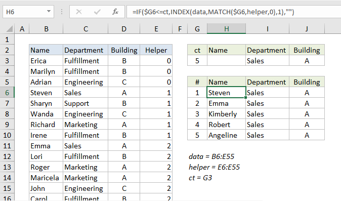
In the example shown, the formula in H6 is:
=IF($G6<=ct,INDEX(data,MATCH($G6,helper,0),1),"")
How this formula works
The challenge with extraction formulas is managing duplicates (i.e. multiple matches). Lookup formulas like VLOOKUP and INDEX + MATCH can easily find the first match, but it’s much harder to lookup “all matches” when criteria select more than one match.
This formula deals with this challenge by using a helper column that returns a numeric value that can be used to easily extract multiple matches.
The formula in the helper column looks like this:
=SUM(E2,AND(C3=$I$3,D3=$J$3))
The helper column tests each row in the data to see if the Department in column C matches the value in I3 and the Building in column D matches the value in J3. Both logical tests must return TRUE in order for AND to return TRUE.
For each row, the result of AND is added to the “value above” in the helper column to generate a count. The practical effect of this formula is an incrementing counter that only changes when a (new) match is found. Then the value remains the same until the next match is found. This works because the TRUE/FALSE results return by AND are coerced to 1/0 values as part of the sum operation. FALSE results add nothing, and TRUE results add 1.
Back in the extraction area, the lookup formula for Name in column H looks like this:
=IF($G6<=ct,INDEX(data,MATCH($G6,helper,0),1),"")
Working from the inside out, the INDEX MATCH part of the formula looks up the name for the first match found, using the row number in column G as the match value:
INDEX(data,MATCH($G6,helper,0),1)
INDEX receives all 3 columns of data as the array (named range “data”), and MATCH is configured to match the row number inside the helper column (the named range “helper”) in exact match mode (3rd argument set to zero).
This is where the cleverness of the formula becomes apparent. The helper column obviously contains duplicates, but it doesn’t matter, because MATCH will match only the first value. By design, each “first value” corresponds to the correct row in the data table.
The formulas in columns I and J are the same as H, except for the column number, which is increased in each case by one.
The IF statement that wraps the INDEX/MATCH formula performs a simple function — it checks each row number in the extraction area to see if the row number is less than or equal to the value in G3 (named range “ct”), which is the total count of all matching records. If so, the INDEX/MATCH logic is run. If not, IF outputs an empty string (“”).
The formula in G3 (named range “ct”) is simple:
=MAX(helper)
Since the maximum value in the helper column is the same as the total match count, the MAX function is all we need.
Note: the extraction area needs to be manually configured to handle as much data as needed (i.e. 5 rows, 10 rows, 20 rows, etc.). In this example, it is limited to 5 rows only to keep the worksheet compact.