Merge tables with VLOOKUP in Excel

This tutorial shows how to  Merge tables with VLOOKUP in Excel using the example below;

Formula

=VLOOKUP($A1,table,COLUMN()-x,0)

Explanation

To merge tables, you can use the VLOOKUP function to lookup and retrieve data from one table to the other. To use VLOOKUP this way, both tables must share a common id or key.

This article explains how join tables using VLOOKUP and a calculated column index. This is one way to use the same basic formula to retrieve data across more than one column.

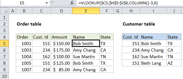
In the example shown, we are using VLOOKUP to  pull Name and State into the invoice data table. The VLOOKUP formula used for both is identical:

=VLOOKUP($C5,$H$5:$J$8,COLUMN()-3,0)

How this formula works

This is a standard “exact match” VLOOKUP formula with one exception: the column index is calculated using the COLUMN function. When the COLUMN function is used without any arguments, it returns a number that corresponds to the current column.

In this case, the first instance of the formula in column E returns 5, since column E is the 5th column in the worksheet. We don’t actually want to retrieve data from the 5th column of the customer table (there are only 3 columns total) so we need to subtract 3 from 5 to get the number 2, which is used to retrieve Name from customer data:

COLUMN()-3 = 2 // column E

When the formula is copied across to column F, the same formula yields the number 3:

COLUMN()-3 = 3 // column F

As a result, the first instance gets Name from the customer table (column 2), and the 2nd instance gets State from the customer table (column 3).

You can use this same approach to write one VLOOKUP formula that you can copy across many columns to retrieve values from consecutive columns in another table.

With two-way match

Another way to calculate a column index for VLOOKUP is to do a two-way VLOOKUP using the MATCH function. With this approach, the MATCH function is used to figure out the column index needed for a given column in the second table.