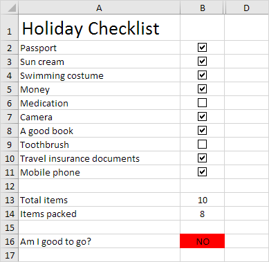
How to create Checklist in Excel

This example teaches you how to  insert checkbox to create a checklist in Excel. First, turn on the Developer tab. Next, you can create a checklist. You can also insert a check mark symbol.

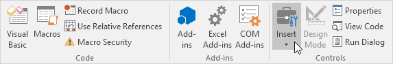
1. On the Developer tab, in the Controls group, click Insert.

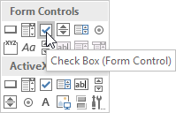
2. Click Check Box in the Form Controls section.

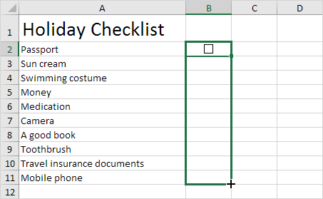
3. Draw a check box in cell B2.

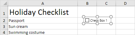
4. To remove “Check Box 1”, right click the check box, click the text and delete it.

5. Select cell B2.

6. Click on the lower right corner of cell B2 and drag it down to cell B11.

7. Right click the first check box and click Format Control.

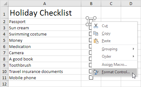
8. Link the check box to the cell next to it (cell C2).

9. Repeat step 8 for the other check boxes.

10. The count the number of items packed, insert a COUNTIF function into cell B14.

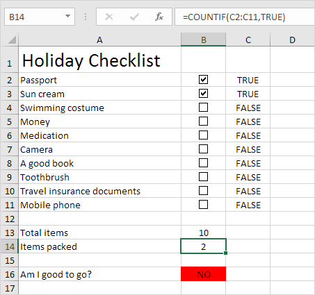
11. Hide column C.

12. Insert an IF function into cell B16.

Result:

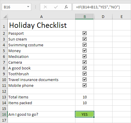
Note: we created a conditional formatting rule to change the background color of cell B16 depending on the cell’s value.