Skip to content
Free Excel Tutorials
  • Home
  • Excel For Beginners
  • Excel Intermediate
  • Advanced Excel For Experts

Data Analysis

  • Add Outline to Data in Excel
  • How To Sort One Column or Multiple Columns in Excel
  • How To Compare Two Lists in Excel
  • Excel Pie Chart
  • How to Create Gantt Chart in Excel

References

  • How to get first row number in range in Excel
  • Perform case-sensitive Lookup in Excel
  • MATCH function: Description, Usage, Syntax, Examples and Explanation
  • Merge tables with VLOOKUP in Excel
  • Basic INDEX MATCH approximate in Excel

Data Validations

  • Excel Data validation date in specific year
  • Excel Data validation unique values only
  • Excel Data validation with conditional list
  • Excel Data validation date in next 30 days
  • Excel Data validation must begin with

Basic error trapping example in Excel

by

To catch errors that a formula might trigger in a worksheet, you can use the IFERROR function to display a custom message, or nothing at all. See example below:

Formula

=IFERROR(formula,value_if_error)

Explanation

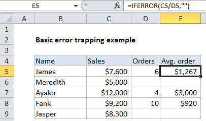
In the example shown, the formula in E5 is:

=IFERROR(C5/D5,"")

How this formula works

In this example, the IFERROR function is used to trap and suppress the #DIV/0! error that occurs when there is no value for Orders (column D). Without IFERROR, the formula C5/D5 would display a #DIV/0! error in E6 and E9.

The IFERROR function takes two arguments: a value (usually entered as a formula), and a result to display if the formula returns an error. The second argument is only used if the first argument throws an error.

In this case, the first argument is the simple formula for calculating the average order size, which divides total sales by the order count:

=C5/D5

The second argument is entered as an empty string (“”).

When the formula returns a normal result, the result is displayed.

When the formula returns #DIV/0!, an empty string is returned and nothing is displayed.

Post navigation

Previous Post:

How to calculate project complete percentage in Excel

Next Post:

Popularly Used Excel Functions and their examples

Leave a Reply Cancel reply

Your email address will not be published. Required fields are marked *

Learn Basic Excel

Ribbon
Workbook
Worksheets
Format Cells
Find & Select
Sort & Filter
Templates
Print
Share
Protect
Keyboard Shortcuts

Categories

  • Charts
  • Data Analysis
  • Data Validation
  • Excel Functions
    • Cube Functions
    • Database Functions
    • Date and Time Functions
    • Engineering Functions
    • Financial Functions
    • Information Functions
    • Logical Functions
    • Lookup and Reference Functions
    • Math and Trig Functions
    • Statistical Functions
    • Text Functions
    • Web Functions
  • Excel VBA
  • Excel Video Tutorials
  • Formatting
  • Grouping
  • Others

Logical Functions

  • How to use Excel OR Function
  • Invoice status with nested if in Excel
  • IFERROR function: Description, Usage, Syntax, Examples and Explanation
  • SWITCH function example in Excel
  • How to return blank in place of #DIV/0! error in Excel

Date Time

  • How to calculate nth day of year in Excel
  • Get fiscal year from date in Excel
  • How to calculate project start date based on end date in Excel
  • Convert text date dd/mm/yy to mm/dd/yy in Excel
  • Convert Excel time to decimal seconds

Grouping

  • Running count group by n size in Excel
  • Group numbers with VLOOKUP in Excel
  • Group times into unequal buckets in Excel
  • Group times into 3 hour buckets in Excel
  • Categorize text with keywords in Excel

General

  • How to calculate percentage of total in Excel
  • How to calculate percent sold in Excel
  • Spell Check in Excel
  • Hide and Unhide Columns or Rows in Excel
  • How to get original price from percentage discount in Excel
© 2026 xlsoffice . All Right Reserved. | Teal Smiles | Abbreviations And Their Meaning