Case sensitive match in Excel

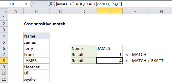
To perform a case sensitive match, you can use the EXACT function together with MATCH in an array formula. In the example show, the formula in E8 is:

{=MATCH(TRUE,EXACT(B5:B11,E6),0)}

Note: this is an array formula and must be entered with Control + Shift + Enter.

How this formula works

By itself, the MATCH function is not case-sensitive, so the following formula returns 1:

=MATCH("JAMES",B5:B11,0)

To add case-sensitivity, we use the EXACT function like this:

EXACT(B5:B11,E6)

Which returns an array of TRUE/FALSE values:

{FALSE;FALSE;FALSE;TRUE;FALSE;FALSE;FALSE}

This array goes into the MATCH function as the lookup_array. For lookup_value, we use TRUE with MATCH set to exact match mode by setting match_type to zero.

=MATCH(TRUE,{FALSE;FALSE;FALSE;TRUE;FALSE;FALSE;FALSE},0)

Match then returns the position of the first TRUE value found: 4.