25 Basic Excel Formulas and Functions Worked Examples

Mastering the basic Excel formulas is critical for beginners to become highly proficient in data analysis.

A formula is an expression which calculates the value of a cell. Functions are predefined formulas and are already available in Excel. Every formula in Excel starts with an equal sign, then the function name and in bracket a cell name or cell ranges or cell references. See illustration below:

=Function Name( cell name or cell ranges or cell references). Let’s begin with simple Arithmetic Operators calculation in Excel such as Addition, Subtraction and multiplication.

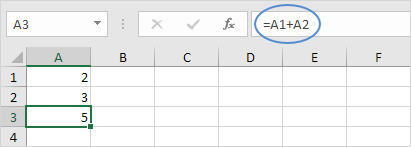
For example, cell A3 below contains a formula which adds the value of cell A2 to the value of cell A1.

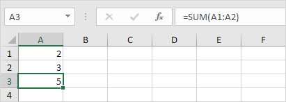
For example, cell A3 below contains the SUM function which calculates the sum of the range A1:A2.

Enter a Formula

To enter a formula, execute the following steps.

1. Select a cell.

2. To let Excel know that you want to enter a formula, type an equal sign (=).

3. For example, type the formula A1+A2.

Tip: instead of typing A1 and A2, simply select cell A1 and cell A2.

4. Change the value of cell A1 to 3.

Excel automatically recalculates the value of cell A3. This is one of Excel’s most powerful features!

Edit a Formula

When you select a cell, Excel shows the value or formula of the cell in the formula bar.

1. To edit a formula, click in the formula bar and change the formula.

2. Press Enter.

Operator Precedence

Excel uses a default order in which calculations occur. If a part of the formula is in parentheses, that part will be calculated first. It then performs multiplication or division calculations. Once this is complete, Excel will add and subtract the remainder of your formula. See the example below.

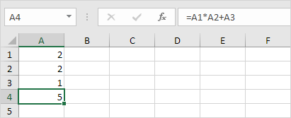
First, Excel performs multiplication (A1 * A2). Next, Excel adds the value of cell A3 to this result.

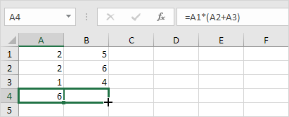
Another example,

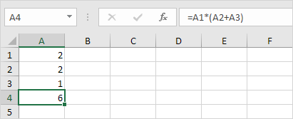
First, Excel calculates the part in parentheses (A2+A3). Next, it multiplies this result by the value of cell A1.

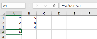
Copy/Paste a Formula

When you copy a formula, Excel automatically adjusts the cell references for each new cell the formula is copied to. To understand this, execute the following steps.

1. Enter the formula shown below into cell A4.

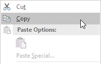
2a. Select cell A4, right click, and then click Copy (or press CTRL + c)…

…next, select cell B4, right click, and then click Paste under ‘Paste Options:’ (or press CTRL + v).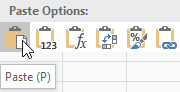

2b. You can also drag the formula to cell B4. Select cell A4, click on the lower right corner of cell A4 and drag it across to cell B4. This is much easier and gives the exact same result!

Result. The formula in cell B4 references the values in column B.

Using Excel in-built functions

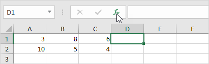
Insert a Function

Every function has the same structure. For example, SUM(A1:A4). The name of this function is SUM. The part between the brackets (arguments) means we give Excel the range A1:A4 as input. This function adds the values in cells A1, A2, A3 and A4. It’s not easy to remember which function and which arguments to use for each task. Fortunately, the Insert Function feature in Excel helps you with this.

To insert a function, execute the following steps.

1. Select a cell.

2. Click the Insert Function button.

The ‘Insert Function’ dialog box appears.

3. Search for a function or select a function from a category. For example, choose COUNTIF from the Statistical category.

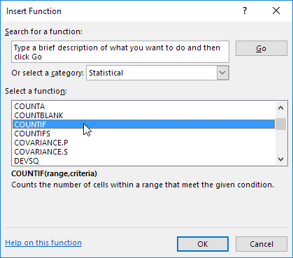
4. Click OK.

The ‘Function Arguments’ dialog box appears.

5. Click in the Range box and select the range A1:C2.

6. Click in the Criteria box and type >5.

7. Click OK.

Result. The COUNTIF function counts the number of cells that are greater than 5.

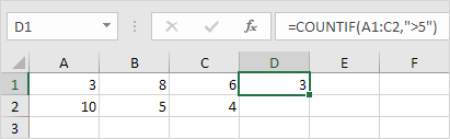
Note: instead of using the Insert Function feature, simply type =COUNTIF(A1:C2,”>5″). When you arrive at: =COUNTIF( instead of typing A1:C2, simply select the range A1:C2.

Worked Example: Sum Function Formula

The SUM() function, as the name suggests, gives the total of the selected range of cell values. It performs the mathematical operation which is addition. Here’s an example of it below:

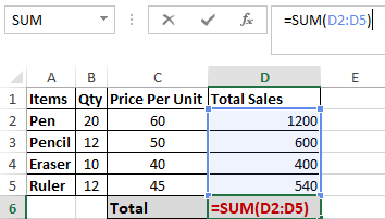
As you can see above, to find the total amount of sales for every unit, we had to simply type in the function “=SUM(D2:C5)”. This automatically adds up 1200, 600, 400 and 540. The result is stored in D6.

Worked Example: Average Function Formula

The AVERAGE() function focuses on calculating the average of the selected range of cell values. As seen from the below example, to find the avg of the total sales, you have to simply type in “AVERAGE(D2, D3, D4,D5)”.

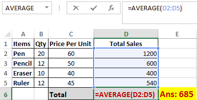
It automatically calculates the average, and you can store the result in your desired location.

Worked Example: Count Function Formula

The function COUNT() counts the total number of cells in a range that contains a number. It does not include the cell, which is blank, and the ones that hold data in any other format apart from numeric.

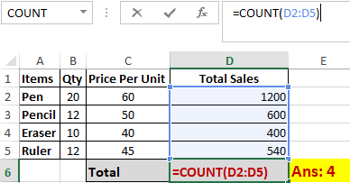
As seen above, here, we are counting from C1 to C4, ideally four cells. But since the COUNT function takes only the cells with numerical values into consideration, the answer is 3 as the cell containing “Total Sales” is omitted here.

Worked Example: Subtotal Function Formula

Moving ahead, let’s now understand how the subtotal function works. The SUBTOTAL() function returns the subtotal in a database. Depending on what you want, you can select either average, count, sum, min, max, min, and others. Let’s have a look at two such examples.

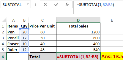
In the example above, we have performed the subtotal calculation on cells ranging from A2 to A4. As you can see, the function used is “=SUBTOTAL(1, B2: B5), in the subtotal list “1” refers to average. Hence, the above function will give the average of B2: B5 and the answer to it is 13.5, which is stored in D6.

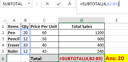
Similarly, “=SUBTOTAL(4, B2: B5)” selects the cell with the maximum value from B2 to B5, which is 20. Incorporating “4” in the function provides the maximum result.

Worked Example: Modulus Function Formula

The MOD() function works on returning the remainder when a particular number is divided by a divisor. Let’s now have a look at the examples below for better understanding.

In the first example, we have divided 20 by 3. The remainder is calculated using the function “=MOD(B2,3)”. The result is stored in B2. We can also directly type “=MOD(20,3)” as it will give the same answer.
modulus

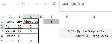
Similarly, here, we have divided 12 by 3. The remainder is 0 is, which is stored in C3.

Worked Example: Power Function Formula

The function “Power()” returns the result of a number raised to a certain power. Let’s have a look at the examples shown below:

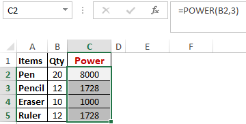
As you can see above, to find the power of 20 stored in B2 raised to 3, we have to type “= POWER (B2,3)”. This is how power function works in Excel.

Worked Example: Ceiling Function Formula

Next, we have the ceiling function. The CEILING() function rounds a number up to its nearest multiple of significance.

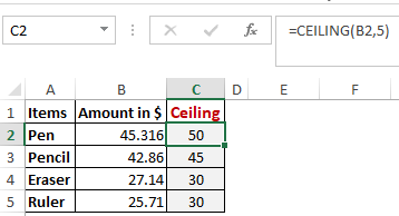
The nearest highest multiple of 5 for 45.316 is 50, 42.86 is 45 and so on.

Worked Example: Floor Function Formula

Contrary to the Ceiling function, the floor function rounds a number down to the nearest multiple of significance.

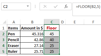
The nearest lowest multiple of 5 for 45.316 is 45.

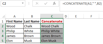
Worked Example: Concatenate Function Formula

This function merges or joins several text strings into one text string. Given below are the different ways to perform this function.

In this example, we have operated with the syntax =CONCATENATE(A25, ” “, B25)
concatenate

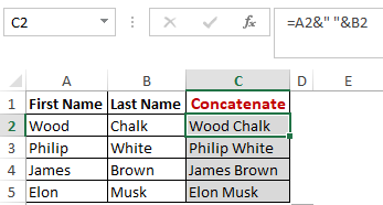
Method 1

Method 2

In this example, we have operated with the syntax using alternate method =A2&” “&B2
concatenate-function.

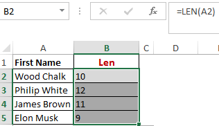
Worked Example: Len Function Formula

The function LEN() returns the total number of characters in a string. So, it will count the overall characters, including spaces and special characters. Given below is an example of the Len function.

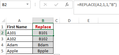
Worked Example: Replace Function Formula

As the name suggests, the REPLACE() function works on replacing the part of a text string with a different text string.

The syntax is “=REPLACE(old_text, start_num, num_chars, new_text)”. Here, start_num refers to the index position you want to start replacing the characters with. Next, num_chars indicate the number of characters you want to replace.

Let’s have a look at the ways we can use this function.

Here, we are replacing A101 with B101 by typing “=REPLACE(A2,1,1,”B”)”.

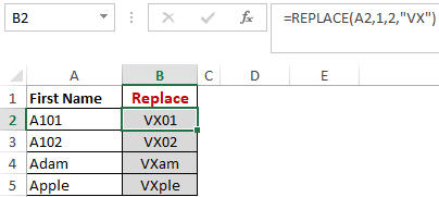
Next, we are replacing A102 with VX102 by typing “=REPLACE(A2,1,1, “VX”)”.

UPPER, LOWER, PROPER

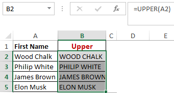
The UPPER() function converts any text string to uppercase. In contrast, the LOWER() function converts any text string to lowercase. The PROPER() function converts any text string to proper case, i.e., the first letter in each word will be in uppercase, and all the other will be in lowercase.

Let’s understand this better with the following examples:

Worked Example: Upper Function Formula

Here, we have converted the text range A2-A5 to Capital Letters in B2-B5.

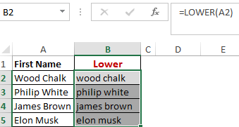
Worked Example: Lower Function Formula

Now, we have converted the text range A2-A5 to Small Letters in B2-B5.

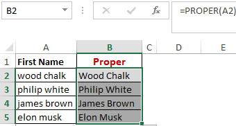
Worked Example: Proper Function Formula

Finally, we have converted the improper text in range A2-A5 to Initial Caps in B2-B5.

Now, let us hop on to exploring some date and time functions in Excel.

LEFT, RIGHT, MID

The LEFT() function gives the number of characters from the start of a text string. Meanwhile, the MID() function returns the characters from the middle of a text string, given a starting position and length. Finally, the right() function returns the number of characters from the end of a text string.

Let’s understand these functions with a few examples.

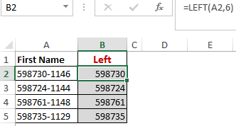
Worked Example: Left Function Formula

In the example below, we use the function left to extract 6 leftmost numbers from the “text string”/numbers in the table.

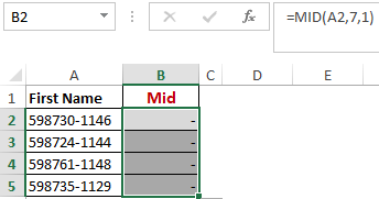
Worked Example: Mid Function Formula

Shown below is an example using the mid function.

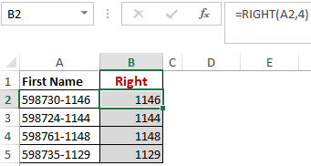
Worked Example: Right Function Formula

Here, we have an example of the right function. The example below, illustrates the use of Right function to extract the last 4 numbers from the right of the “text string”/numbers in the table.

Worked Example: Now() Function Formula

The NOW() function in Excel gives the current system date and time.

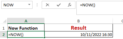
The result of the NOW() function will change based on your system date and time.

Worked Example: Today() Function Formula

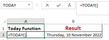
The TODAY() function in Excel provides the current system date.

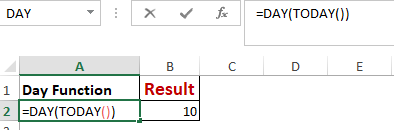
Worked Example: Day() Function Formula

The function DAY() is used to return the day of the month. It will be a number between 1 to 31. 1 is the first day of the month, 31 is the last day of the month.

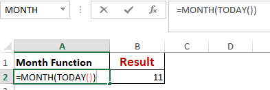
Worked Example: Month() Function Formula

The MONTH() function returns the month, a number from 1 to 12, where 1 is January and 12 is December.

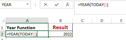
Worked Example: Year() Function Formula

The YEAR() function, as the name suggests, returns the year from a date value.

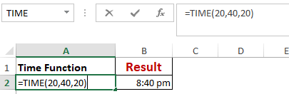
Worked Example: Time() Function Formula

The TIME() function converts hours, minutes, seconds given as numbers to an Excel serial number, formatted with a time format.

HOUR, MINUTE, SECOND

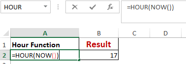
Worked Example: Hour() Function Formula

The HOUR() function generates the hour from a time value as a number from 0 to 23. Here, 0 means 12 AM and 23 is 11 PM.

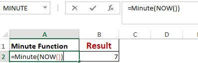
Worked Example: Minute() Function Formula

The function MINUTE(), returns the minute from a time value as a number from 0 to 59.

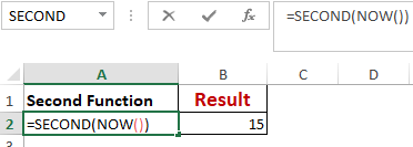
Worked Example: Second() Function Formula

The SECOND() function returns the second from a time value as a number from 0 to 59.

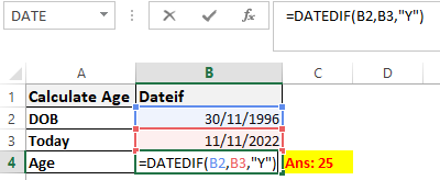
Worked Example: Datedif Function Formula

The DATEDIF() function provides the difference between two dates in terms of years, months, or days.

Below is an example of a DATEDIF function where we calculate the current age of a person based on two given dates, the date of birth and today’s date.