How to fill cell ranges with random text values in Excel

To quickly fill a range of cells with random text values, you can use a formula based on the CHOOSE and RANDBETWEEN functions.

Formula

=CHOOSE(RANDBETWEEN(1,3),"Value1","Value2","Value3")

Note that RANDBETWEEN will calculate a new value whenever the worksheet is changed. Once you have values in the range, you may want to replace the formulas with values to prevent further changes.

Explanation

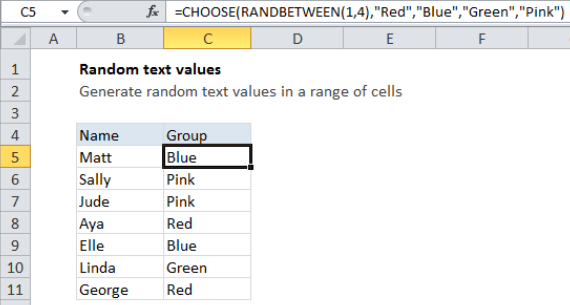
In the example shown, the formula in C5 is:

=CHOOSE(RANDBETWEEN(1,4),"Red","Blue","Green","Pink")

Which returns a random color from the values provided.

How this formula works

The CHOOSE function provides the framework for this formula. Choose takes a single numeric value as its first argument (index_number), and uses this number to select and return one of the values provides as subsequent arguments, based on their numeric index.

In this case, we are using four values: Red, Blue, Green, and Pink, so we need to give CHOOSE a number between 1 and 4.

To generate this number, we use RANDBETWEEN, a function that returns a random integer between a bottom and top value. Since we are only working with 4 values in CHOOSE, we supply 1 for the bottom number and 4 for the top number.

When this formula is copied down, it will return one of the four colors.